hpmicrosimr modelling vignette

hpmicrosimr is an agent-based model of residential energy efficiency retrofits. This is a development, but fully operational, version of hpmicrosimr that tracks space heating upgrade choices by $\approx 800$ Irish owner-occupier households or “agents”. Agent characteristics are based on survey data collected in late 2024. The model runs at bi-monthly time-steps by default. It is initialised at the beginning of 2015 and is calibrated to historical data over the period 2015-2025. The outputs of hpmicrimsimr are intended to represent the pre-2015 Irish housing stock of about 1.16M households.

The main elements of hpmicrosimr are:

1. a financial model of the household return on residential energy efficiency investment
2. an initialiser that generates a partially randomised initial state with missing data is imputed
3. an updater that generates agents energy efficiency choices in the time-step $t$, $t+\Delta t$.
4. a run module where the user inputs a policy scenario

The financial model in hpmicrosimr is based on “equivalent annual cost” (EAC). EAC is the sum of $opex$ (heating bills and maintenance costs) and an annualised capital cost. The annualised capital cost depends on the agents time preferences (discount rate $r$), the cost of the heating technology, the cost of building fabric upgrades, state grant supports, fuel prices etc. The heating systems included in the current version of hpmicrosimr are oil, solid_fuel, gas, electric and air source heat_pumps. At present, it is assumed that the space heating requirement is fully satisfied by the primary heating source, and therefore secondary and tertiary heat sources do not play a role in the current model.

Two distinct stochastic processes are simulated in the updater. Process 1 describes the random failure and replacement of the current heating technology. The failure probability depends on the age of the heating system, based on a Weibull hazard function with technology-specific parameters consistent with engineering data. When the current heating system fails, agents choose either to replace it with the original technology or to adopt a heat pump. For simplicity, hpmicrosimr excludes other switching possibilities e.g. gas to oil. A critical feature that lowers uptake is that a heat pump may be rejected even when it appears to offer a lower EAC. For instance, a household whose oil or gas boiler has failed might determine that $\Delta EAC = EAC_{\rm{reject}} - EAC_{\rm{adopt}} > 0$. This is insufficient for adoption in hpmicrosimr unless the financial advantage exceeds a heterogeneous threshold $$\begin{equation} \frac{\Delta EAC}{EAC_{\mathrm{reject}}} > \theta \tag{1} \end{equation}$$ The heterogeneity of the “barrier” $\theta$, representing risk aversion and other factors, is determined from a micro-calibration to the survey data. When an existing heat pump fails, hpmicrosimr assumes that the agents choose between replacement with a new heat pump or switching to gas. There is no $\theta$ barrier in this case, but on the other hand no grant support is available. Historical improvements in boiler efficiency mean that Process 1 leads to a gradual improvement in residential energy efficiency (BER) even in the absence of heat pumps.

Peer effects can lower the barrier to adoption of a heat pump in Equation (1). The survey data show that having an associate who has already installed a heat pump increases the stated likelihood to adopt. The number of associates with whom households share information related to energy efficiency is also known from the survey. This peer effect is captured in hpmicrosimr by placing the agents on an assortative social influence network where the degree distribution matches the survey. A new random social network is generated for each model run.

In Process 2, some randomly selected subset of agents decide to evaluate energy efficiency improvements (Building Energy Rating, BER). This reflects a desire to save money and/or to improve home comfort. The investment decision optimises the choice of building fabric upgrade and heating technology choice. The optimum upgrade depends on the initial and final values of the Heat Loss Indicator ($HLI$). A function hpmicrosimr::optimise_upgrade() determines the optimum upgrade in terms of technology and $HLI$ improvement, including state grant incentives that apply at model time $t$.

The rate at which households choose to update the energy efficiency of their home in Process 2 is set by an “inertia” parameter $p.$, i.e. the fraction of agents, randomly selected, who choose to evaluate home energy efficiency improvement in the current time interval. If the value of $p.$ is small and energy costs are high, most households have not yet taken advantage of energy efficiency upgrades that could reduce their costs, giving rise to a so-called energy efficiency “gap” or “paradox”. In addition, barriers such as the “hassle” associated with $HLI$ upgrades may also contribute to the energy efficiency gap. Along with other poorly determined parameters, $p.$ must be found from macro-calibration of hpmicrosimr to historical grant uptake data (2015-2025).

Table 1 summarises the “behavioural” adjustments to EAC implemented in hpmicrosimr that influence agents’ energy efficiency choices. The agents time preferences are described by two parameters- a discount rate $r$ and a present bias $\beta$. Present bias lowers the benefit of future energy bill savings relative to the investment cost. In addition, Table 1 has a parameter related to an aversion to household disruption $\eta$ caused by deep energy retrofits and an aversion to making grant applications $\tau$. There is also a large “prebound effect” $\rho$ quantifying the underheating of very inefficient buildings.

Table 1: Calibration Parameters

parameter	symbol	typical_value	type	source
risk aversion	θ	10-30%	heterogeneous barrier	survey (2024)
discount rate	r	3.5%	homogeneous	macro-calibration
present bias	β	0.5	homogeneous	calibration
inertia	p	0.05	homogeneous	calibration
disruption	η	0.16	homogeneous	calibration
sludge	τ	0.02	homogeneous	calibration
prebound	ρ	0.4	homogeneous	observed FEC

The cost of alternative heating technologies is evaluated using:

$$\begin{equation} EAC = opex + \frac{CRF(r)}{\beta} (capex-grant) \tag{2} \end{equation}$$ where $CRF(r)$ is the capital reduction factor. A heat pump is adopted provided that the EAC of a heat pump evaluated using Equation (2) is sufficiently low relative to the maintaining the current technology, Equation (1). Present bias $\beta$ makes heat pumps less favourable because of their much higher $capex$, but grants mitigate this effect.

Process 2 involves the decision whether or not to upgrade the building fabric. Neglecting behavioural adjustments, the change in EAC due to an investment in fabric upgrade would be:

$$\begin{equation} \Delta EAC = \Delta opex + r(capex - grant) \tag{3a} \end{equation}$$ Comparing to Equation (2), $HLI$ improvements are assumed to be long-lived so that $CRF(r) = r$. $\Delta opex$ is the reduction in annual bills calculated from the change in engineering space heating requirement following the upgrade. hpmicrosimr uses the expression: $$\begin{equation} \Delta opex = 52.7 \frac{\Delta HLI}{\epsilon} p_{fuel} \tag{4} \end{equation}$$ where $\epsilon$ is the heating system efficiency (i.e. $\epsilon < 1$ for boilers and $\approx$ 3 for a heat pump ) and $p_{fuel}$ is the prevailing fuel price in units $€/kWh$. Equation (4) assumes a standard Heating Degree Days of 2,196 $^\circ C-\mathrm{days}$ for Ireland. Note that a prebound effect $\rho$ is not included in Equation (4). The reason is that part of the return on investment in building fabric upgrades comes in the form of improved comfort. The return calculated using the engineering space heating requirement captures the full welfare gain for the agent include financial cost and comfort. On the other hand, a calculation of the impact on actual bills or energy consumption would need to take prebound into effect.

In reality, Equation (3a) does not describe the observed uptake of building fabric retrofits because it tends to favour deep energy retrofits. In practice, most grants are for shallower refits which is inconsistent with Equation (3a). This suggests that Equation (3a) should be modified to account for the significant impact of non-financial factors $\beta$, $\eta$ and $\tau$. hpmicrosimr makes the plausible assumption that disruption effect scales with capital cost ($\eta \times capex$) and the grant application “sludge” scales with grant size ($\tau \times grant$). Equation (3a) becomes:

$$\begin{equation} \Delta EAC = \Delta opex + \left(\frac{r}{\beta} + \eta \right) capex - \left(\frac{r}{\beta} - \tau \right) grant \tag{3b} \end{equation}$$ Equation (3b) with the parameter values of Table 1 gives a good description of the observed cumulative grant uptake by scheme and measure (heat pumps and fabric upgrades) over the period 2015-2025. Note that the disruption effect is larger that the direct financial cost.

Heating System Cost Model

hpmicrosimr assumes that the heating technology costs are linear in the installed capacity $C= A+ B \times kW_{peak}$ with technology-specific parameters $A$ and $B$. $kW_{peak}$ is the peak design load (coldest day) and is linear in $HLI$. For example, hpmicrosimr gives a design capacity of 8.3 kW for a 100m$^2$ house with $HLI=2.3$. The implied cost of a replacement gas boiler is €2,100, while the cost of a new heat pump is €10,500.

Fabric Ugrade Cost Model

Detailed approaches to fabric upgrade costs consider individual building elements and housing archetypes. hpmicromsimr uses a simplified model derived from an underlying marginal cost model. The marginal cost for $HLI$ upgrades crosses over from low cost measures for incremental improvements in inefficient buildings, to a very high marginal costs for a building that is already efficient. $$\begin{equation} \frac{d C}{d HLI} = \frac{c_{min}}{1+e^{-\left(HLI-HLI_0\right)/k}} + \frac{c_{max}}{1+e^{\left(HLI-HLI_0\right)/k}} \tag{5a} \end{equation}$$$C$ is the upgrade cost for a 100m$^2$ floor area. Equation (5a) can be integrated to find the cost for an upgrade from $HLI_{i}$ to $HLI_{f}$$$\begin{equation} C(HLI_i,HLI_f) = c_{max} \left(HLI_{old}-HLI_{new}\right) + K\left(c_{max}-c_{min}\right) \log{\left[ \frac{1+e^{(HLI_{f}-HLI_0)/k})}{1+e^{(HLI_{i}-HLI_0)/k}} \right]} \tag{5b} \end{equation}$$ Appropriate parameter values in Equation (5b) are determined from reported upgrade costs and case studies. They depend on house type and region. For example, for a two-storey, semi-detached house in Munster, $c_{min}= €42{ {^}C}m2/W $, $c_{max}= €465 { ^\circ}C{m^2}/W$. The cross-over scale is $K=0.37W/{ {^\circ} C}{m^2}$. The location of the crossover $HLI_0 = 2.3 W/{ ^\circ C}{m^2}$ corresponds to a BER of C2 for a house with a modern efficient condensing gas boiler.

Figure 1 illustrates Equation (4b). Note the steeply rising costs for upgrades of already efficient buildings versus the “low hanging fruit” available for upgrades of inefficient buildings.

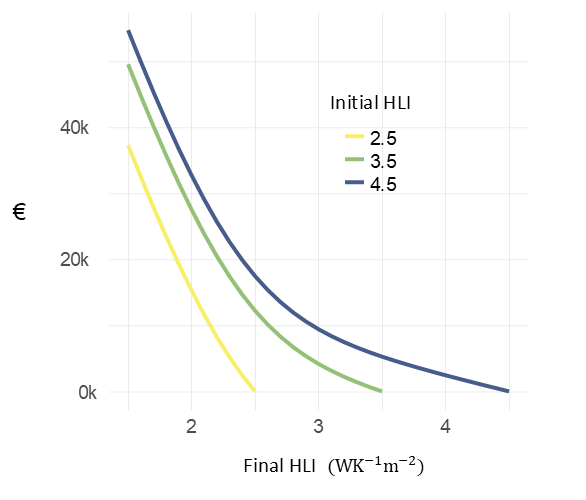
Figure 1: Fabric Upgrade cost curves

Optimal upgrade

Equations (3b), (4) and (5a) can be used to find the optimal fabric upgrade, given the current $HLI_{initial}$. For the special case where the cost is fully covered by the grant (no financial disincentive), the optimal $EAC$ is given by the solution of $$\begin{equation} \left(\eta + \tau\right ) MC(HLI_{final}) = \frac{52.7 p_f}{\epsilon} \tag{6} \end{equation}$$ where $HLI_{final} < HLI_{initial}$. Therefore if the “hassle” $\eta + \tau > 52.7p_f/\epsilon MC(HLI_{initial})$, no fabric upgrade is undertaken. If the fuel price is $0.12/kWh$, $\epsilon = 0.9$.

Scenarios

Applications of hpmicrosimr are to project energy efficiency outcomes based on future policy scenarios (such as WEM/WAM), impacts on CO2 emissions, and associated cost-benefit analysis of generous incentive schemes.

A separate package hpmicrocalibrater is used to generate the model weights and thresholds and are provided in a dataset agents_init.

Calibration